Neural Networks
Loading Packages
using DataFrames, CSV, ScikitLearn, PyPlotLoading the dataset
data = CSV.File("covid_cleaned.csv") |> DataFrame20352×16 DataFrame
Row │ intubed pneumonia age pregnancy diabetes copd asthma inmsupr hypertension other_disease cardiovascular obesity renal_chronic tobacco contact_other_covid covid_res
│ Int64 Int64 Int64 Int64 Int64 Int64 Int64 Int64 Int64 Int64 Int64 Int64 Int64 Int64 Int64 Int64
───────┼──────────────────────────────────────────────────────────────────────────────────────────────────────────────────────────────────────────────────────────────────────────────────────
1 │ 0 0 25 0 0 0 0 0 0 0 0 0 0 0 1 1
2 │ 0 0 52 0 0 0 0 0 0 0 0 1 0 1 1 1
3 │ 0 1 51 0 0 0 0 0 0 0 0 0 0 0 1 1
4 │ 1 1 67 0 1 0 0 0 1 0 0 1 0 0 1 1
5 │ 0 1 59 0 1 0 0 0 0 0 0 0 0 0 1 1
6 │ 0 0 52 0 1 0 0 0 1 0 1 0 0 0 0 1
7 │ 0 1 54 0 0 0 0 0 0 0 0 0 0 0 0 1
8 │ 0 1 78 0 0 0 0 0 1 0 0 1 0 0 1 1
⋮ │ ⋮ ⋮ ⋮ ⋮ ⋮ ⋮ ⋮ ⋮ ⋮ ⋮ ⋮ ⋮ ⋮ ⋮ ⋮ ⋮
20346 │ 1 1 65 0 0 0 0 0 0 0 0 0 0 0 0 0
20347 │ 0 1 49 0 0 0 0 0 0 0 0 0 0 0 0 0
20348 │ 0 1 80 0 1 0 0 0 0 0 0 0 0 0 0 0
20349 │ 0 0 13 0 0 0 0 0 0 0 0 0 0 0 0 0
20350 │ 1 0 23 0 0 0 0 0 0 1 0 0 0 1 0 0
20351 │ 0 1 1 0 0 0 0 0 0 0 0 0 0 0 0 0
20352 │ 0 1 55 0 0 0 0 0 0 0 0 1 0 0 0 0
20337 rows omittedThe ScikitLearn package only accepts the data in array form, hence we need to convert our data into Arrays
X = convert(Array, data[!,Not(:covid_res)])
y = convert(Array, data[!,:covid_res]) # :covid_res is our target variable
Splitting the data into training set and test set
@sk_import model_selection: train_test_split
X_train, X_test, y_train, y_test = train_test_split(X, y, test_size=0.33, random_state=42) # You can define the train/test size ratio using the test_size argumenttrain_test_splitis a function provided by the scikit-learn package.If you want random sampling while splitting the data, assign a number the the
random_stateargument to thetrain_test_splitfunction.test_sizespecifies what should be the ratio of test data in the collection after splitting the data into training set and test set. Here we have specified that we need a test dataset of size = 33% of the original data.
Model Definition
@sk_import neural_network: MLPClassifier
mlp_6layer = MLPClassifier(hidden_layer_sizes=(30, 50, 60, 10, 10, 10))
In this example we are using a NN Classifier. A Neural Network Regressor can be defined by
MLPRegressor.The number of layers and number of nodes are defined by values passed to
hidden_layer_sizes. Here we are saying that we need 6 hidden layers with 1st layer having 30 nodes, 2nd layer having 50 nodes, 3rd layer having 60 nodes, 4th, 5th, and 6th layer having 10 layers.
Model Fitting
fit!(mlp_6layer,X_train,y_train)This will fit your model to the training dataset.
Model Evaluation
Classification report with the training data:
y_pred = predict(mlp_6layer,X_train)

@sk_import metrics: classification_report
print(classification_report(y_train,y_pred))
> precision recall f1-score support
0 0.65 0.51 0.57 5684
1 0.70 0.80 0.75 7951
accuracy 0.68 13635
macro avg 0.67 0.66 0.66 13635
weighted avg 0.68 0.68 0.67 13635Classification report with the test data:
y_pred = predict(simplelogistic,X_test)
print(classification_report(y_test,y_pred))
> precision recall f1-score support
0 0.65 0.52 0.57 2763
1 0.70 0.80 0.75 3954
accuracy 0.69 6717
macro avg 0.68 0.66 0.66 6717
weighted avg 0.68 0.69 0.68 6717Cross Validation
@sk_import model_selection: cross_val_score
cross_val_score( MLPClassifier(hidden_layer_sizes=(30, 50, 60, 10, 10, 10)), X_train, y_train)5-element Array{Float64,1}:
0.6651998533186652
0.6681334800146681
0.658965896589659
0.6729006233956729
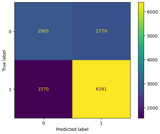
0.6802346901356803Confusion Matrix
@sk_import metrics: plot_confusion_matrix
plot_confusion_matrix(mlp_6layer,X_train,y_train)
PyPlot.gcf()