Mathematical Foundations of the PGDCM Bayesian Network Model

Introduction

At the heart of the pgdcm package lies a single, unified Bayesian network model defined in the file DiBelloBN.R. This one piece of NIMBLE code is highly flexible: depending on how you configure your graph (i.e., which node types and compute rules you assign), it can express a standard Diagnostic Classification Model (DCM), an Item Response Theory (IRT) model, a Multidimensional IRT (MIRT) model, or a Higher-Order DCM (HO-DCM).

This vignette is written for readers who want to understand exactly what the model is doing mathematically. We will walk through:

1. The general equation that governs every node in the network.
2. The three condensation rules (DINA, DINO, DINM) that determine how parent information is combined.
3. How the model specializes into IRT, MIRT, DCM, and HO-DCM depending on the graph topology.
4. The semantic meaning of every estimated parameter.

---

1. The Big Picture: Everything is a Bayesian Network

A pgdcm model is a Directed Acyclic Graph (DAG) - a network of nodes connected by directional arrows, with no cycles. There are two kinds of nodes:

• Attribute nodes (latent/unobserved): These represent skills, abilities, or competencies that we cannot directly see. For example, “Addition” or “Reading Comprehension.” We want to estimate whether each student has mastered these.
• Task nodes (observed): These represent actual test items (questions). We can see whether each student answered correctly (1) or incorrectly (0).

The arrows (edges) in the graph encode dependency: if there is an arrow from Attribute $A$ to Task $T$, it means that mastery of $A$ influences the probability of answering $T$ correctly. If there is an arrow from Attribute $A_1$ to Attribute $A_2$, it means that $A_1$ is a prerequisite for $A_2$.

The question that every model must answer is: Given the pattern of correct/incorrect responses we observe, what is the most likely configuration of latent skills for each student?

Topological Ordering

Because the graph is acyclic, we can always arrange nodes in a topological order - an ordering where every parent appears before its children. The pgdcm package enforces this automatically via enforce_topo_sort(). This ordering is critical because it means we can process nodes from left to right: when we reach any node, all of its parents have already been defined.

The nodes are ordered as:

$$\underbrace{\alpha_1, \alpha_2, \ldots, \alpha_K}_{\text{Attribute nodes}} \;,\; \underbrace{X_1, X_2, \ldots, X_J}_{\text{Task nodes}}$$

where $K$ is the number of attributes and $J$ is the number of items.

---

2. The Universal Equation: Logistic Regression at Every Node

Every node in the network (whether an attribute or a task) follows the same fundamental equation. The probability that node $v$ “fires” (equals 1) for student $i$ is:

$$P(v_i = 1) = \text{logit}^{-1}\!\Big(\underbrace{a_v}_{\text{slope}} \cdot \underbrace{\psi_v(\text{parents of } v)}_{\text{condensation rule}} - \underbrace{b_v}_{\text{intercept}}\Big)$$

Let us unpack each piece:

2.1 The Logistic (Inverse-Logit) Function

The logistic function $\text{logit}^{-1}(x) = \frac{1}{1 + e^{-x}}$ transforms any real number into a probability between 0 and 1. It is the standard “link” function in logistic regression:

Input $x$	$\text{logit}^{-1}(x)$
$-5$	$\approx 0.007$
$-2$	$\approx 0.12$
$0$	$0.50$
$+2$	$\approx 0.88$
$+5$	$\approx 0.993$

When the input is large and positive, the probability approaches 1. When it is large and negative, the probability approaches 0. At $x = 0$, the probability is exactly $0.50$.

2.2 The Slope ($a_v$): Discrimination

The slope (also called the discrimination parameter) controls how sharply the probability transitions from low to high as the condensed input changes. Think of it as the “sensitivity” of the node:

• A large slope (e.g., $a_v = 5$) means the node is very good at discriminating between students who have the prerequisite skills and those who do not. The probability jumps rapidly from near 0 to near 1.
• A small slope (e.g., $a_v = 0.5$) means the node is a weak discriminator - even students with all the right skills only have a moderately higher probability of success.

In the pgdcm code, item slopes are stored in lambda[j, 1] and attribute transition slopes are stored in theta[k, 1]. They are constrained to be positive via a truncated normal prior $\text{TN}(\mu, \sigma, 0, \infty)$, ensuring that more skill always means higher probability (never inverted).

2.3 The Intercept ($b_v$): Difficulty / Base-Rate

The intercept controls the baseline difficulty of the node - how hard it is to “pass” when the condensation rule ($\psi_v$) outputs exactly zero.

Specifically:

• When $\psi_v = 0$, the probability resolves to $\text{logit}^{-1}(-b_v)$.
• A large positive $b_v$ means the node is difficult: the baseline probability of success is low (it is hard to guess, or hard for an average student).
• A large negative $b_v$ means the node is easy: the baseline probability of success is high.
• At $b_v = 0$, the baseline probability is exactly 0.50.

In the code, item intercepts are lambda[j, 2] and attribute intercepts are theta[k, 2].

Why the Minus Sign?

Notice the equation uses $a_v \cdot \psi_v - b_v$ and not $a_v \cdot \psi_v + b_v$. The minus sign is a psychometric convention that makes $b_v$ directly interpretable as difficulty: higher $b_v$ = harder item. If we used a plus sign, a positive $b_v$ would make the item easier, which is less intuitive. You will see this convention in most IRT textbooks.

2.4 The Condensation Rule ($\psi_v$): Combining Parent Information

Each node has one or more parent nodes (the nodes with arrows pointing into it). The condensation rule $\psi_v$ takes all the parent values and collapses them into a single number that the logistic regression uses as input.

The condensation rule is computed by the calc_mixed_kernel() function. There are three options:

Rule	Name	Compute Value	Cognitive Interpretation
DINA	Deterministic Input, Noisy “And”	"dina"	All-or-nothing: Student must have every required skill
DINO	Deterministic Input, Noisy “Or”	"dino"	Any-one-sufficient: Having at least one skill is enough
DINM	Deterministic Input, Noisy “Mixed”	"dinm"	Proportional: Each additional skill incrementally helps

We detail each rule in the next section.

---

3. The Three Condensation Rules (Pure Discrete Case)

To build intuition, let us first consider the pure discrete case - where all parent attributes are binary (0 or 1). We will extend to continuous parents later.

Suppose item $j$ requires skills $\alpha_1$ and $\alpha_2$ (indicated by 1s in the corresponding Q-matrix row).

3.1 DINA: The Conjunctive (“And”) Gate

The DINA rule asks: Does the student possess ALL required skills?

$$\psi_j^{\text{DINA}} = \prod_{k \in \text{parents}(j)} \alpha_{ik}^{q_{jk}} = \begin{cases} 1 & \text{if the student has mastered every required skill} \\ 0 & \text{otherwise} \end{cases}$$

where $q_{jk}$ is the Q-matrix entry (1 if skill $k$ is required for item $j$, 0 otherwise) and $\alpha_{ik}$ is student $i$’s mastery state (0 or 1) on skill $k$.

Example: Item 5 requires skills $A$ and $B$.

Student	$\alpha_A$	$\alpha_B$	$\psi^{\text{DINA}}$	Interpretation
Alice	1	1	1	Has both skills → high chance of success
Bob	1	0	0	Missing skill B → treated exactly like having no skills
Carol	0	0	0	Missing both → low chance of success

The DINA rule is strict: mastering 3 out of 4 required skills is treated identically to mastering 0 out of 4. There is no partial credit for partial mastery.

In the code, this is computed as:

gate <- (sum_disc == req_disc)   # Are all required discrete skills present?
val_dina <- gate                 # 1 if yes, 0 if no

With the full logistic equation, the probabilities become:

• All skills present ($\psi = 1$): $P = \text{logit}^{-1}(a \cdot 1 - b) = \text{logit}^{-1}(a - b)$
• Any skill missing ($\psi = 0$): $P = \text{logit}^{-1}(a \cdot 0 - b) = \text{logit}^{-1}(-b)$

The gap between these two probabilities is controlled by the slope $a$. A large slope creates a wide gap, meaning the item can clearly distinguish masters from non-masters.

3.2 DINO: The Disjunctive (“Or”) Gate

The DINO rule asks: Does the student possess AT LEAST ONE required skill?

$$\psi_j^{\text{DINO}} = 1 - \prod_{k \in \text{parents}(j)} (1 - \alpha_{ik})^{q_{jk}} = \begin{cases} 1 & \text{if the student has mastered at least one required skill} \\ 0 & \text{if the student has mastered none of the required skills} \end{cases}$$

Example: Same item requiring skills $A$ and $B$:

Student	$\alpha_A$	$\alpha_B$	$\psi^{\text{DINO}}$	Interpretation
Alice	1	1	1	Has both → high chance
Bob	1	0	1	Has one → still high chance
Carol	0	0	0	Has none → low chance

DINO is lenient: having just one of the required skills is as good as having all of them. This models scenarios where multiple skills each independently provide a path to the correct answer.

In the code:

dino_gate <- 0.0
if (sum_disc > 0.0) {
    dino_gate <- 1.0        # At least one skill is present
}
val_dino <- dino_gate

3.3 DINM: The Compensatory (Proportional) Rule

The DINM rule asks: What fraction of the required skills does the student possess?

$$\psi_j^{\text{DINM}} = \frac{\sum_{k} q_{jk} \cdot \alpha_{ik}}{\sum_{k} q_{jk}}$$

This produces a value between 0 and 1, representing the proportion of required skills mastered.

Example: Same item requiring skills $A$ and $B$:

Student	$\alpha_A$	$\alpha_B$	$\psi^{\text{DINM}}$	Interpretation
Alice	1	1	$2/2 = 1.0$	Has all skills → highest probability
Bob	1	0	$1/2 = 0.5$	Has half → moderate probability
Carol	0	0	$0/2 = 0.0$	Has none → lowest probability

DINM provides partial credit: each additional skill smoothly increases the probability of success. This is the most “forgiving” model in terms of rewarding partial knowledge.

In the code:

val_dinm <- sum_total / max(1, sum_input)

---

4. Root Attributes: Base-Rates and Latent Abilities

Every DAG has root nodes - nodes with no incoming arrows (no parents). In a pgdcm model, these are the “foundational” attributes. How they are modeled depends on an important configuration flag: isContinuousHO.

4.1 Standard Discrete Roots (isContinuousHO = 0)

When root attributes are discrete, each one is treated as an independent Bernoulli variable with its own base-rate probability. The model estimates a single parameter $\beta_m$ for each root attribute $m$:

$$P(\alpha_{im} = 1) = \text{logit}^{-1}(-\beta_m)$$

Since this is a root node (no parents, no condensation rule), the probability depends only on the intercept $\beta_m$. This parameter represents the population-level difficulty of mastering this skill:

• $\beta_m = 0$: the skill is mastered by about 50% of the population.
• $\beta_m > 0$ (positive): the skill is mastered by fewer than 50% - it is a difficult skill.
• $\beta_m < 0$ (negative): the skill is mastered by more than 50% - it is an easy/common skill.

In the code, this parameter is beta_root[m], with a normal prior:

beta_root[m] ~ dnorm(mean = beta_prior_mean[m, 1], sd = beta_prior_std[m, 1])

4.2 Continuous Roots (isContinuousHO = 1)

When root attributes are continuous, they represent latent abilities rather than binary mastery states. Each student’s ability on dimension $m$ is drawn from a standard normal distribution:

$$\alpha_{im} \sim \mathcal{N}(0, 1)$$

This is the standard identification constraint used in IRT: fixing the mean to 0 and the variance to 1 ensures the model is identifiable (otherwise, we could shift and scale the ability axis without changing any observable quantity). In this case, no beta_root parameter is estimated - the ability values themselves are directly estimated for each student.

Importantly, the rest of the model doesn’t change. When these continuous values flow into child nodes through the condensation rules, the logistic equation naturally adapts.

---

5. Case Studies: How the Graph Topology Creates Different Models

Now we show how simply changing the graph structure-without altering any model code-creates fundamentally different psychometric models.

5.1 Traditional DCM (Flat Q-Matrix)

Graph structure:

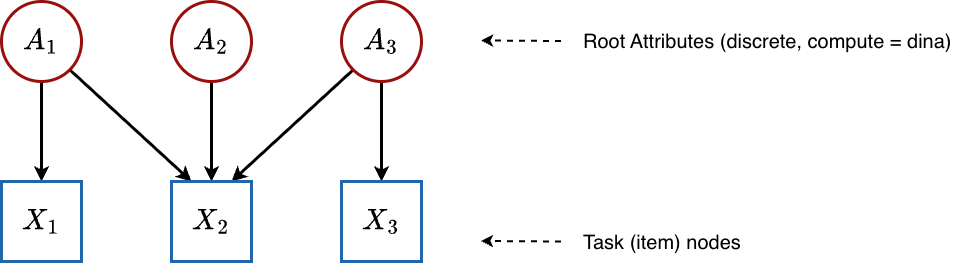
All attributes are roots (no arrows between attributes), and they point directly to the items. This is the classic Q-matrix structure.

Configuration: All attributes have compute = "dina" and isContinuousHO = 0.

What happens mathematically:

1. Root attributes: Each skill $\alpha_k$ is an independent Bernoulli variable: $$P(\alpha_{ik} = 1) = \text{logit}^{-1}(-\beta_k) \quad \text{for } k = 1, \ldots, K$$

2. Items: There are no dependent attributes (no hierarchy). Each item uses the condensation rule directly: $$P(X_{ij} = 1 \mid \boldsymbol{\alpha}_i) = \text{logit}^{-1}\!\left(\lambda_{j1} \cdot \psi_j(\boldsymbol{\alpha}_i) - \lambda_{j2}\right)$$

The specific form of $\psi_j$ depends on which compute rule the item is assigned. For a flat DINA Q-matrix with items requiring skills $\{A_1, A_2\}$:

$$\psi_j^{\text{DINA}} = \alpha_{i,1} \cdot \alpha_{i,2}$$

Estimated parameters:

Parameter	Symbol	Count	Meaning
beta_root[m]	$\beta_m$	$K$	Population mastery rate of each root skill
lambda[j, 1]	$\lambda_{j1}$	$J$	Item discrimination (how separable the masters vs. non-masters are)
lambda[j, 2]	$\lambda_{j2}$	$J$	Item difficulty (baseline challenge level)
attributenodes[i, k]	$\alpha_{ik}$	$N \times K$	Each student’s binary mastery state on each skill

Note that theta parameters are absent in this flat case. The theta parameters only exist for dependent (non-root) attributes - nodes that have parent attributes feeding into them. Since all attributes here are independent roots, there are no attribute-to-attribute transitions to parameterize.

5.2 Hierarchical DCM / Bayesian Net DCM (Discrete Attribute Hierarchy)

Graph structure:

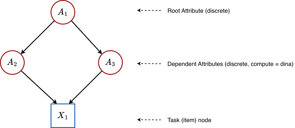
Some attributes depend on other attributes. For example, “Multiplication” might require “Addition” as a prerequisite. Here, $A_1$ is a root (no parents), while $A_2$ and $A_3$ are dependent attributes that receive input from $A_1$.

Configuration: All attributes have compute = "dina" and isContinuousHO = 0, but the graph contains edges between attributes.

What happens mathematically:

1. Root attribute: $A_1$ is modeled exactly as before: $$P(\alpha_{i1} = 1) = \text{logit}^{-1}(-\beta_1)$$

2. Dependent attributes: Each non-root attribute $A_k$ gets its own theta parameters. The condensation rule $\psi_k$ summarizes the parent skill values, and then a logistic regression determines mastery: $$P(\alpha_{ik} = 1 \mid \text{parents}) = \text{logit}^{-1}(\theta_{k,1} \cdot \psi_k - \theta_{k,2})$$

   Here:

   • $\theta_{k,1}$ (theta[k, 1]) is the transition slope - how strongly mastery of the parent skills influences whether the student masters skill $k$. A large value means that parent mastery is highly predictive of child mastery.
   • $\theta_{k,2}$ (theta[k, 2]) is the transition intercept - the baseline difficulty of mastering skill $k$, independent of parent skills. A large positive value means this skill is hard to acquire even when all parent skills are mastered.

3. Items: Same as the flat case - items see the binary attribute values and apply the condensation rule + lambda parameters.

Estimated parameters:

Parameter	Symbol	Count	Meaning
beta_root[m]	$\beta_m$	$K_{\text{root}}$	Population mastery rate of each root skill
theta[k, 1]	$\theta_{k,1}$	$K - K_{\text{root}}$	How strongly parent skills predict mastery of dependent skill $k$
theta[k, 2]	$\theta_{k,2}$	$K - K_{\text{root}}$	Baseline difficulty of acquiring dependent skill $k$
lambda[j, 1]	$\lambda_{j1}$	$J$	Item discrimination
lambda[j, 2]	$\lambda_{j2}$	$J$	Item difficulty
attributenodes[i, k]	$\alpha_{ik}$	$N \times K$	Each student’s binary mastery state on each skill

This is the case where theta parameters first appear - whenever attributes have parent attributes, the model needs parameters to describe those transitions.

5.3 Unidimensional IRT (Single Continuous Root)

Graph structure:

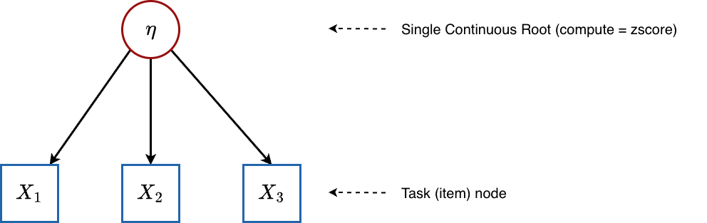
A single latent ability $\eta$ directly influences all items. There are no discrete skills.

Configuration: Single attribute with compute = "zscore" and thus isContinuousHO = 1.

What happens mathematically:

1. Root attribute (ability): For each student $i$: $$\eta_i \sim \mathcal{N}(0, 1)$$

2. Items: Each item receives $\eta_i$ as its only input through the condensation rule. Since there is one continuous parent and no discrete parents, the DINA condensation rule simplifies to: $$\psi_j = \eta_i$$ (The “gate” is open because there are no discrete skills to check.)

   The item response probability becomes: $$P(X_{ij} = 1 \mid \eta_i) = \text{logit}^{-1}(\lambda_{j1} \cdot \eta_i - \lambda_{j2})$$

This is exactly the Two-Parameter Logistic (2PL) IRT model:

$$P(X_{ij} = 1 \mid \eta_i) = \frac{1}{1 + \exp\!\big(-\big(a_j \cdot \eta_i - b_j\big)\big)}$$

where $a_j = \lambda_{j1}$ is the item discrimination and $b_j = \lambda_{j2}$ is the item difficulty.

Estimated parameters:

Parameter	Symbol	Count	Meaning
lambda[j, 1]	$a_j$	$J$	Item discrimination - how steeply the item’s probability curve rises with ability
lambda[j, 2]	$b_j$	$J$	Item difficulty - the ability level at which a student has a 50% chance of success (when $a_j = 1$)
attributenodes[i, 1]	$\eta_i$	$N$	Each student’s latent ability (a continuous real number, centered at 0)

Interpreting the Difficulty Parameter $b_j$ in IRT

In the 2PL parameterization $P = \text{logit}^{-1}(a(\eta - b))$, the difficulty $b_j$ is the point on the ability scale where a student has exactly 50% probability of success. The pgdcm parameterization uses $a\eta - b$ rather than $a(\eta - b)$, so the “50% point” occurs at $\eta = b/a$ rather than exactly $\eta = b$. This is a common alternative parameterization found in many Bayesian IRT implementations.

No beta_root or theta parameters are estimated in IRT mode - there are no discrete roots (so no beta_root) and no dependent attributes (so no theta).

5.4 Multidimensional IRT (MIRT)

Graph structure:

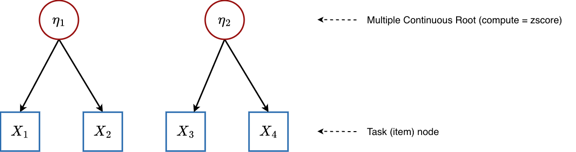
Multiple continuous latent abilities, each influencing a subset of items.

Configuration: Multiple attributes with compute = "zscore", giving isContinuousHO = 1 and nrbetaroot > 1.

What happens mathematically:

1. Root attributes (abilities): For each student $i$ and dimension $m$: $$\eta_{im} \sim \mathcal{N}(0, 1)$$

2. Items: An item may depend on one or more ability dimensions. The condensation rule sums the contributions from all relevant continuous parents. For example, if item $j$ depends on both $\eta_1$ and $\eta_2$: $$\psi_j = q_{j1} \cdot \eta_{i1} + q_{j2} \cdot \eta_{i2}$$

   So: $$P(X_{ij} = 1 \mid \boldsymbol{\eta}_i) = \text{logit}^{-1}\!\left(\lambda_{j1} \cdot \left(\sum_{m} q_{jm} \, \eta_{im}\right) - \lambda_{j2}\right)$$

This produces a compensatory MIRT model where multiple dimensions contribute additively. Item discrimination $\lambda_{j1}$ scales the total ability input, while individual dimension loadings are encoded in the Q-matrix structure.

Estimated parameters:

Parameter	Symbol	Count	Meaning
lambda[j, 1]	$a_j$	$J$	Overall item discrimination (how strongly the item discriminates on the combined ability)
lambda[j, 2]	$b_j$	$J$	Item difficulty
attributenodes[i, m]	$\eta_{im}$	$N \times M$	Each student’s ability on each continuous dimension

5.5 Higher-Order DCM (HO-DCM)

Graph structure:

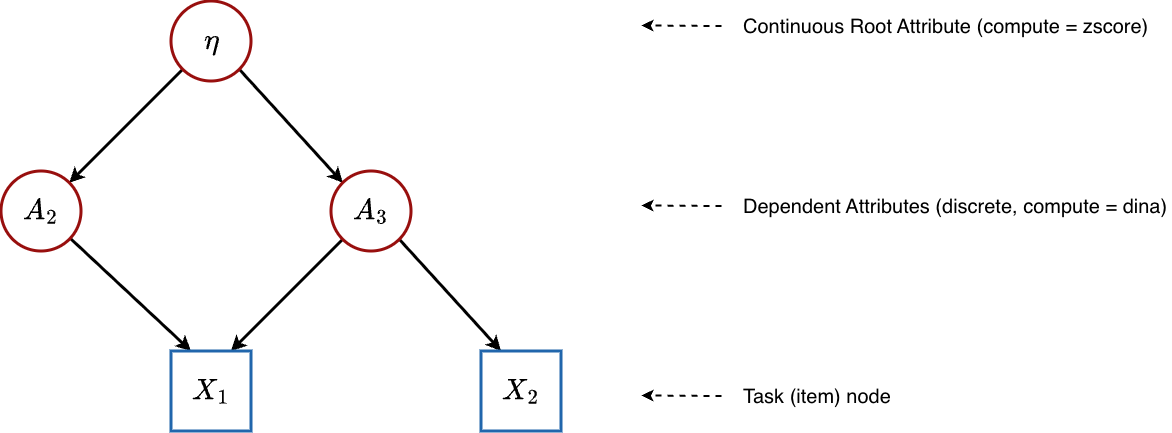
A single continuous general ability $\eta$ feeds into discrete binary skills, which in turn determine item responses.

Configuration: Root attribute has compute = "zscore" (continuous), child attributes have compute = "dina" (discrete). This gives isContinuousHO = 1.

What happens mathematically:

This model type demonstrates the full mixed continuous-discrete capability of DiBelloBN. The network has three layers:

Layer 1 - General Ability (Root): $$\eta_i \sim \mathcal{N}(0, 1)$$

Layer 2 - Discrete Skills (Dependent Attributes):

Each dependent attribute $A_k$ depends on the general ability $\eta$ through a logistic regression. The condensation rule passes $\eta_i$ straight through:

$$\psi_k = \eta_i$$

The probability that student $i$ has mastered skill $k$:

$$P(\alpha_{ik} = 1 \mid \eta_i) = \text{logit}^{-1}(\theta_{k1} \cdot \eta_i - \theta_{k2})$$

where:

• $\theta_{k1}$ (stored as theta[k, 1]) is the transition slope for skill $k$. It controls how sensitive skill mastery is to changes in general ability $\eta$. A large value means that small differences in general ability produce large differences in the probability of mastering this skill. A small value means the skill is only weakly related to general ability.
• $\theta_{k2}$ (stored as theta[k, 2]) is the transition intercept (threshold) for skill $k$. It determines the baseline difficulty of acquiring the skill. A student with general ability $\eta_i$ has a 50% chance of mastering skill $k$ when $\theta_{k1} \cdot \eta_i = \theta_{k2}$, i.e., at the ability level $\eta_i = \theta_{k2} / \theta_{k1}$. A larger $\theta_{k2}$ means the student needs higher general ability to have a reasonable chance of mastering the skill.

Layer 3 - Items (Observed):

Item responses depend on the discrete skill states $\alpha_{ik}$. Since the roots are continuous but items may only see the discrete child attributes, the condensation rule at this level operates on purely discrete inputs (the binary skill values):

$$P(X_{ij} = 1 \mid \boldsymbol{\alpha}_i) = \text{logit}^{-1}(\lambda_{j1} \cdot \psi_j^{\text{DINA}}(\boldsymbol{\alpha}_i) - \lambda_{j2})$$

The nrbetaroot trick in the code (isContinuousHO * nrbetaroot) ensures that at the item level, the model correctly treats the skill values as discrete, even though $\eta$ was originally continuous. Only the roots themselves “know” they are continuous; the items only see the binary $\alpha_k$ values that resulted from thresholding $\eta$ through the skill-level logistic regressions.

Estimated parameters:

Parameter	Symbol	Count	Meaning
attributenodes[i, 1]	$\eta_i$	$N$	General latent ability for each student
theta[k, 1]	$\theta_{k1}$	$K-1$	Transition slope: sensitivity of skill mastery to general ability
theta[k, 2]	$\theta_{k2}$	$K-1$	Transition intercept: difficulty threshold for acquiring the skill
lambda[j, 1]	$\lambda_{j1}$	$J$	Item discrimination
lambda[j, 2]	$\lambda_{j2}$	$J$	Item difficulty
attributenodes[i, k]	$\alpha_{ik}$	$N \times (K-1)$	Binary mastery states for each specific skill

Why Higher-Order Models?

In a flat DCM, skills are estimated independently - the model does not know or care whether a student who masters “Addition” is also likely to master “Subtraction.” A higher-order model introduces explicit statistical dependence: skills that load heavily on general ability will be correlated in the posterior. This produces more realistic skill profiles and can improve estimation accuracy when skills are genuinely related.

---

6. The Gated Condensation Rule: Handling Mixed Parents

What happens when a node has both continuous and discrete parents? This arises naturally in a Bayesian network where a continuous root ($\eta$) and discrete attributes ($A_1, A_2$) all point to the same child node.

The calc_mixed_kernel() function handles this with a gating mechanism:

1. Separate the parents into continuous parents (indices $\leq$nrbetaroot) and discrete parents (indices $>$nrbetaroot).
2. Check the gate (specific to DINA or DINO).
3. If the gate is open, pass the continuous signal through.
4. If the gate is closed, apply a severe penalty ($-10$), which drives the logistic probability to near zero.

Gated DINA (Mixed Non-Compensatory)

$$\psi^{\text{Gated-DINA}} = \begin{cases} \underbrace{\sum_{m \leq M_{\text{root}}} q_{jm} \cdot \eta_{im}}_{\text{sum of continuous inputs}} & \text{if all required discrete skills are mastered} \\[8pt] -10 & \text{otherwise (gate closed)} \end{cases}$$

Semantic meaning: The student must first pass the discrete skills “gatekeeper.” Only if they possess every required binary skill does their continuous ability actually count. Otherwise, no amount of general ability can help - the gate is shut.

Gated DINO (Mixed Disjunctive)

$$\psi^{\text{Gated-DINO}} = \begin{cases} \sum_{m \leq M_{\text{root}}} q_{jm} \cdot \eta_{im} & \text{if at least one required discrete skill is mastered} \\[8pt] -10 & \text{otherwise (gate closed)} \end{cases}$$

Semantic meaning: The student needs any one of the required binary skills to unlock the gate. Once any skill is present, the continuous ability flows through.

DINM with Mixed Parents

The DINM rule does not use gating at all. It simply takes the weighted average across all parents (continuous and discrete alike):

$$\psi^{\text{DINM}} = \frac{\sum_k q_{jk} \cdot \text{parent}_k}{\sum_k q_{jk}}$$

This naturally handles the mix: continuous values contribute proportionally alongside discrete (0/1) values.

Why $-10$ as the Closed-Gate Penalty?

The value $-10$ is not arbitrary - it is chosen so that $\text{logit}^{-1}(a \cdot (-10) - b)$ is vanishingly small for any reasonable slope $a > 0$. For example, with $a = 1$ and $b = 0$: $\text{logit}^{-1}(-10) \approx 0.0000454$. This effectively forces the probability to zero without requiring special-case logic in the NIMBLE model code.

---

7. The Complete Prior Structure

Every unknown parameter in the model is given a prior distribution - a mathematical statement of our beliefs before seeing any data. The priors in DiBelloBN are:

Root Attribute Intercepts (Discrete Mode)

$$\beta_m \sim \mathcal{N}(\mu_{\beta_m}, \sigma_{\beta_m}) \quad \text{for } m = 1, \ldots, K_{\text{root}}$$

Default: $\mu = 0$, $\sigma = 2$. This is a relatively uninformative prior centered at 50% mastery rate, allowing the data to speak.

Attribute Transition Parameters (Dependent Attributes)

$$\theta_{k,1} \sim \text{TN}(\mu_{\theta_{k,1}}, \sigma_{\theta_{k,1}}, 0, \infty) \quad \text{(slope, positive only)}$$$$\theta_{k,2} \sim \mathcal{N}(\mu_{\theta_{k,2}}, \sigma_{\theta_{k,2}}) \quad \text{(intercept)}$$

The truncated normal $\text{TN}(\cdot, \cdot, 0, \infty)$ ensures slopes are positive - more prerequisite mastery should always increase (never decrease) the probability of mastering the dependent skill.

Item Parameters

$$\lambda_{j,1} \sim \text{TN}(\mu_{\lambda_{j,1}}, \sigma_{\lambda_{j,1}}, 0, \infty) \quad \text{(discrimination, positive only)}$$$$\lambda_{j,2} \sim \mathcal{N}(\mu_{\lambda_{j,2}}, \sigma_{\lambda_{j,2}}) \quad \text{(difficulty)}$$

Same logic: discrimination must be positive so that skill mastery always benefits the student.

Customizing Priors

You can control all priors through the priors argument in build_model_config():

# Option 1: Set uniform priors across all parameters
config <- build_model_config(g, X, priors = list(
    beta = c(0, 2),      # mean, sd for all beta_root
    theta = c(0, 2),     # mean, sd for all theta (slope and intercept)
    lambda = c(0, 2)     # mean, sd for all lambda (slope and intercept)
))

# Option 2: Set per-parameter priors using matrices
config <- build_model_config(g, X, priors = list(
    lambda_mean = matrix(c(1, 0,    # Item 1: slope prior mean = 1, intercept prior mean = 0
                           1, 0,    # Item 2
                           1, 0),   # Item 3
                         nrow = 3, byrow = TRUE),
    lambda_std = matrix(0.0001, nrow = 3, ncol = 2)  # Very tight → locks parameters (scoring mode)
))

---

8. Summary: How One Model Becomes Many

The following table summarizes how the same DiBelloBN code adapts to different psychometric models purely through graph configuration:

Model	Root Attributes	Root Compute	Dependent Attributes	Item Compute	Key Parameters
Traditional DCM	$K$ discrete	"dina"	None	"dina" / "dino" / "dinm"	$\beta_m$, $\lambda_{j,1}$, $\lambda_{j,2}$
Bayesian Net DCM	$\geq 1$ discrete	"dina"	$\geq 1$ discrete	"dina" / "dino" / "dinm"	$\beta_m$, $\theta_{k,1}$, $\theta_{k,2}$, $\lambda_{j,1}$, $\lambda_{j,2}$
IRT (2PL)	1 continuous	"zscore"	None	"dina"	$\lambda_{j,1}$, $\lambda_{j,2}$, $\eta_i$
MIRT	$M$ continuous	"zscore"	None	"dina"	$\lambda_{j,1}$, $\lambda_{j,2}$, $\eta_{im}$
HO-DCM	1 continuous	"zscore"	$K$ discrete	"dina" / "dino" / "dinm"	$\theta_{k,1}$, $\theta_{k,2}$, $\lambda_{j,1}$, $\lambda_{j,2}$, $\eta_i$, $\alpha_{ik}$

The entire switching logic is governed by two things:

1. Graph topology - which nodes are roots, which are dependent, and which are tasks.
2. The compute attribute on each node - "dina", "dino", "dinm", or "zscore"/"continuous".

The build_model_config() function inspects these properties and generates the appropriate NIMBLE constants, initial values, and monitors. The model code itself never changes.

---

9. Appendix: Quick Reference - Parameter Mapping

When you run map_pgdcm_parameters() after estimation, pgdcm translates the internal NIMBLE parameter names into human-readable labels. Here is the mapping:

NIMBLE Parameter	Readable Name	Type
beta_root[m]	{Attribute_m} - Prior/Intercept	Root Structure
theta[k, 1]	{Attribute_k} - Dependency on Parent	Attribute Structure (Slope)
theta[k, 2]	{Attribute_k} - Intercept	Attribute Structure (Threshold)
lambda[j, 1]	{Task_j} - Slope	Item Parameter (Discrimination)
lambda[j, 2]	{Task_j} - Intercept	Item Parameter (Difficulty)
attributenodes[i, k]	{Student_i} - {Attribute_k}	Student Mastery